Code
#|label: import-libraries
#|code-fold: true
# Import libraries
library(terra)
library(sf)
library(here)
library(testthat)
library(tmap)
library(kableExtra)
library(tidyverse)
library(dplyr)
#|label: import-libraries
#|code-fold: true
# Import libraries
library(terra)
library(sf)
library(here)
library(testthat)
library(tmap)
library(kableExtra)
library(tidyverse)
library(dplyr)As the global population continues to rise, so does the pressure on wild fisheries to meet growing seafood demand. Marine aquaculture offers a promising solution, providing a sustainable alternative that can relieve pressure on wild stocks while supporting economic development. According to Gentry et al. (2017), the availability of suitable ocean space is unlikely to limit the expansion of marine aquaculture, indicating that many regions have the physical capacity to support future growth. This presents an important opportunity for countries such as the United States to develop aquaculture systems that meet both economic and environmental objectives. Thus, the central objective of this project is to identify which areas along the U.S. West Coast meet the environmental conditions necessary to support sustainable aquaculture development.
Identifying where aquaculture can be responsibly developed requires evaluating the environmental conditions that support healthy growth and minimize ecological impacts. This project assesses the suitability of West Coast Exclusive Economic Zones (EEZs), defined as marine areas extending up to 200 nautical miles from the U.S. coastline where the United States has jurisdiction over natural resource use (NOAA, 2024), for marine aquaculture using two key environmental constraints: sea surface temperature (SST) and bathymetry. Using satellite-derived SST data from 2008–2012 and a regional bathymetry dataset, the total area within each EEZ that meets species-specific environmental thresholds can be quantified. The analysis focuses on two groups: oysters, which are already widely cultivated in California, and the Purple Hinged Rock Scallop (Crassadoma gigantea), a giant scallop species with emerging aquaculture potential (Culver et al., 2022). By integrating spatial environmental data with habitat requirements, this project identifies where conditions are most favorable for expanding sustainable marine aquaculture along the U.S. West Coast.
To assess aquaculture suitability along the U.S. West Coast, a generalized function was implemented that automates the processing of sea surface temperature (SST), bathymetry, and EEZ boundary data. Depth requirements for the purple-hinged rock scallop (Crassadoma gigantea) were obtained from SeaLifeBase, which reports an ecological depth range of 0–80 m below sea level (b.s.l.) (University of British Columbia, 2025; Harbo, 1997). Thermal tolerance data for this species are not provided in SeaLifeBase, so temperature thresholds were derived from Reef Life Survey observations, which indicate a temperature range of approximately 13.3–22.1 degrees Celsius (Schmid, 2025). In addition, suitability thresholds for oysters were incorporated based on published ecological ranges, with optimal SST values between 11–30 degrees Celsius and depth values between 0 and 70 meters b.s.l. These values were used to define species-specific suitability thresholds for reclassification of SST and bathymetry data. The workflow consisted of four phases.
Daily 5-km SST averages from 2008–2012 were compiled and converted into a single long-term mean SST raster. The datasets were first stacked and then averaged by pixel. SST values, originally in Kelvin, were converted to degrees Celsius.
# Load and process SST
SST_2008 <- rast(here('data', 'average_annual_sst_2008.tif'))
SST_2009 <- rast(here('data', 'average_annual_sst_2009.tif'))
SST_2010 <- rast(here('data', 'average_annual_sst_2010.tif'))
SST_2011 <- rast(here('data', 'average_annual_sst_2011.tif'))
SST_2012 <- rast(here('data', 'average_annual_sst_2012.tif'))

# Check that all SST rasters share the same CRS
if (crs(SST_2008) == crs(SST_2009) &
    crs(SST_2009) == crs(SST_2010) &
    crs(SST_2010) == crs(SST_2011)&
    crs(SST_2011) == crs(SST_2012)) {
  print("All coordinate reference systems match!")
} else {
  warning("Coordinate reference systems do not match!")
}

# Stack SST rasters (2008–2012)

sst_stack <- c(SST_2008, SST_2009, SST_2010, SST_2011, SST_2012)

# Check that rasters were stacked successfully
if (!nlyr(sst_stack) > 0) {
     message("SST stack failed: no raster layers detected.")
     stop("Halting execution.")
}

# Compute mean SST over time (per pixel)

mean_sst <- terra::mean(sst_stack)

# Convert temperature units from Kelvin to Celsius

mean_sst_c <- mean_sst - 273.15A regional depth raster was reprojected to match the SST coordinate reference system (CRS). The bathymetry was cropped to the spatial extent of the SST data and resampled to its resolution to maintain consistency and cell alignment between rasters.
# Prepare bathymetry (depth) raster

  # Load the bathymetry raster
bathy <- rast(here("data", "depth.tif"))

# Make CRS match SST:

bathy_proj <- project(bathy, crs(mean_sst_c))

# Check that the re-projection of the depth raster was successful
test_that("Bathymetry CRS matches SST CRS after projection", {
  expect_identical(crs(bathy_proj), crs(mean_sst_c))
})

# Crop bathymetry to SST's extent

bathy_crop <- crop(bathy_proj, mean_sst_c)

# Check resolution of depth vs sst data
if (xres(bathy_crop) == xres(mean_sst_c) &
    (yres(bathy_crop) == yres(mean_sst_c))) {
  print("Raster resolutions match!")
} else {
  warning("Raster resolutions do not match.")
}
Warning: Raster resolutions do not match.# Resample bathymetry to SST resolution (so each cell lines up):
depth_res <- resample(bathy_crop, mean_sst_c, method = "near")
# Check that the depth and SST match in resolution
test_that("Depth raster was resampled to match SST resolution", {
expect_equal(res(depth_res), res(mean_sst_c))
})Species-specific temperature and depth constraints were translated into binary suitability surfaces. For the purple-hinged rock scallop (Crassadoma gigantea), SST values between 13.3–22.1 Celsius and depths between 0–80 meters b.s.l. were classified as suitable (value = 1), with all other values set to unsuitable (value = 0). In contrast, for oysters, suitability was defined by a broader SST range of 11–30 degrees Celsius and shallower depths between 0 and 70 meters b.s.l. Separate binary rasters were generated for each species, and suitability layers were multiplied to produce combined indices identifying locations that simultaneously satisfied both environmental conditions.
# Reclassify SST into suitable / unsuitable
# The oyster thresholds for SST are between 11–30 Celsius

sst_rcl <- matrix(c(-Inf, 11,  0,
                      11, 30,  1,
                      30, Inf, 0), ncol = 3, byrow = TRUE)

sst_suit <- classify(mean_sst_c, rcl = sst_rcl)


# Reclassify depth into suitable or unsuitable (1, 0)
# The depth thresholds for oysters range is 0-70 meters b.s.l.

depth_rcl <- matrix(c(-Inf, -70, 0,
                         -70, 0, 1,
                         0, Inf, 0), ncol = 3, byrow = TRUE)

depth_suit <- classify(depth_res, depth_rcl)

# Combine SST and depth suitability

# Unit test for sst and depth CRS
test_that("Reclassified rasters share identical CRS", {
  expect_identical(crs(sst_suit), crs(depth_suit))
})

# Multiply to get 1 only where both are suitable
suitability <- sst_suit * depth_suit # 1 = suitable, 0 = unsuitableExclusive Economic Zone (EEZ) boundaries were transformed to match the SST projection. The combined suitability raster was masked to the extent of each EEZ, and the area of each raster cell was computed in square kilometers. Suitable cell areas were aggregated within each EEZ to obtain total suitable area per region. These results were subsequently merged with the EEZ polygon dataset and visualized using a colorblind-friendly continuous color scale.
# Prepare EEZ vector and mask
eez_sf <- st_read(here("data", "wc_regions_clean.shp"), quiet = TRUE)

# convert to SpatVector format
eez <- vect(eez_sf)

# Re-project with mean sst's CRS
eez_proj <- project(eez, mean_sst_c)

# Check that the re-projection of the EEZ shapefile was successful
test_that("Bathymetry CRS matches SST CRS after projection", {
  expect_identical(crs(eez_proj), crs(mean_sst_c))
  })

# Mask suitability by EEZ
suitability_eez <- mask(suitability, eez_proj)

# Count suitable cells per EEZ

# a. Compute area in squared kilometers of each raster cell
cell_area_km <- cellSize(suitability_eez, unit = "km")

# b. Multiply suitability (0/1) by area to get "suitable area per cell"
suitable_area_raster <- suitability_eez * cell_area_km
# Cells that were 1 now contain area in km²
# Cells that were 0 remain 0

# c. Extract total suitable area (km²) for each EEZ polygon
eez_suitable_area <- terra::extract(suitable_area_raster,
                             eez_proj,
                             fun = sum,
                             na.rm = TRUE)

# d. Add the EEZ region names to the output
# Replace "region" with the correct column name from your EEZ shapefile
eez_suitable_area$region <- eez_proj$rgn

# Rename the "mean"column
names(eez_suitable_area)[2] <- "suitable_km2"

# Format the table for EEZ suitable area totals
eez_suitable_area_table <- eez_suitable_area %>%
  select(region, suitable_km2) %>%
  kable(col.names = c("EEZ Region", "Suitable Area (km²)"),
        caption = "Total Suitable Area by EEZ Region",
        align = "lr", digits = 1) %>%
  kable_styling(
    full_width = FALSE,
    bootstrap_options = c("striped", "hover"))

# Merge table back into EEZ SpatVector
eez_map <- eez_proj
eez_map$suitable_km2 <- eez_suitable_area$suitable_km2

# Create the final map
map_final <- tm_basemap("Esri.OceanBasemap") +

  tm_shape(eez_map) +

  tm_polygons(fill = "suitable_km2",
              fill.scale = tm_scale_intervals(values = "brewer.blues",
                                              style = "quantile"),
              fill.legend = tm_legend(bg.color = "white",
                                      bg.alpha = 0.2,
                                      title = "Suitable Area (km²)",
                                      frame = FALSE,
                                      position = tm_pos_in("right", "top")),
              col = "black",
              lwd = 0.2) +

  tm_text("rgn", col = "black", fontface = "bold", size = 0.7) +

  tm_title(size = 1,
    text = "Suitable Area for Oyster Aquaculture in West Coast EEZ") +

  tm_layout(frame = TRUE, frame.lwd = 0.4, frame.r = 0) +

  tm_scalebar(breaks = c(0, 250, 500),
              position = tm_pos_in("left", "bottom")) +

  tm_compass(type = "arrow", position = tm_pos_in("left", "top")) +

tmap_options(component.autoscale = FALSE)The workflow was first applied to oysters to demonstrate the processing steps before generalizing the approach. To avoid repeating the oyster workflow for each species, we implemented a generalized function that accepts species-specific parameters.
#|label: oyster-function
source(here("R","suitability_function.R"))

oyster_results <- map_suitability(tmin = 11, tmax = 30,
                                  dmin = -70, dmax = 0,
                                  species_name = "Oysters")
We then tested the function with scallop parameters to confirm that the function can be applied to any species of interest and their ecological parameters.
#|label: scallop-function
scallop_results <- map_suitability(tmin = 13.3, tmax = 22.1,
                                   dmin = -80, dmax = 0,
species_name = "Purple-Hinged Rock Scallops")The resulting suitability maps and EEZ-level summaries for oysters and scallops are shown below.
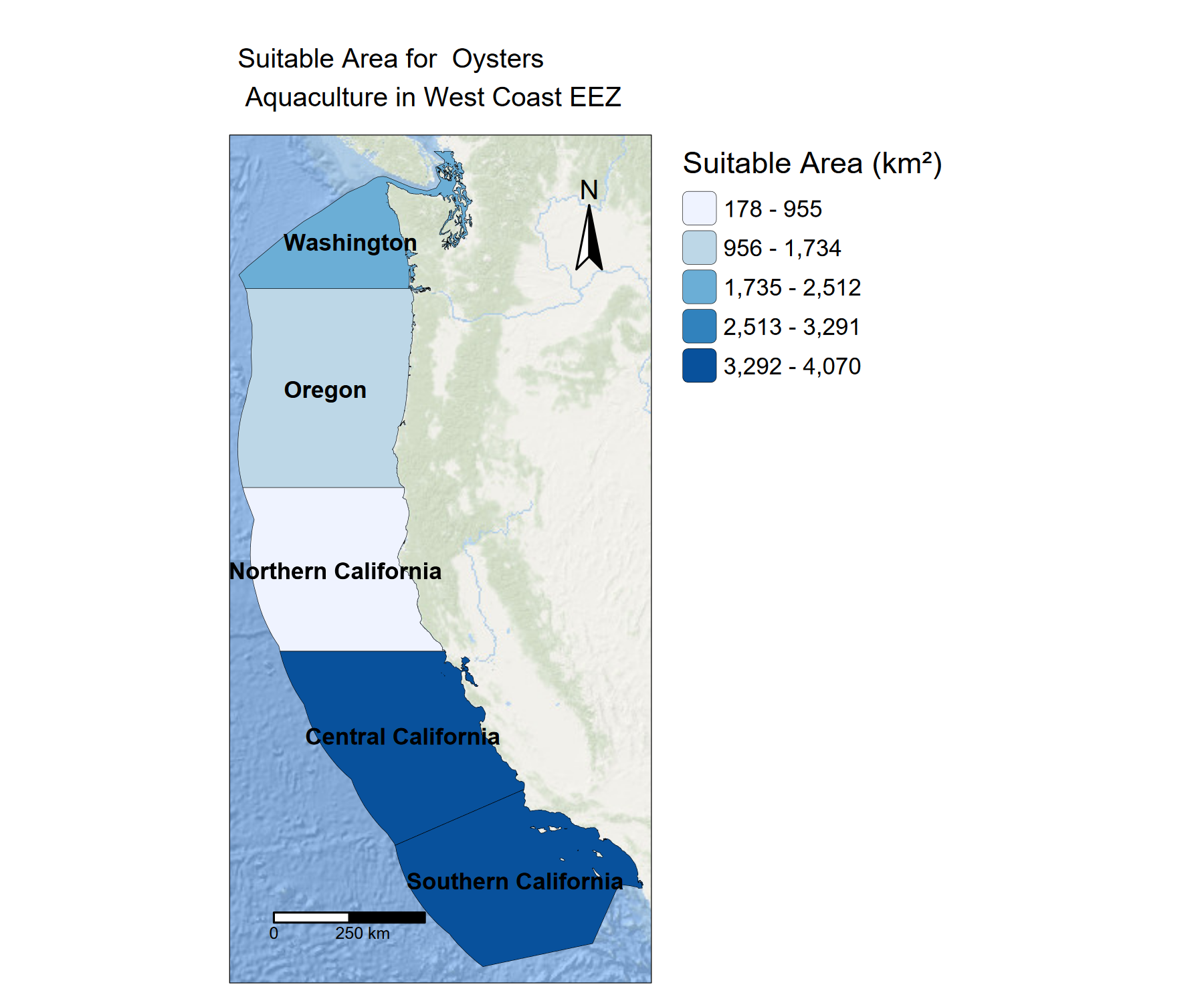
To support comparisons across regions, the total environmentally suitable area for aquaculture within each West Coast Exclusive Economic Zone (EEZ) is summarized in the figures below. These tables quantify how much space within each EEZ meets species-specific temperature and depth thresholds. With these metrics, aquaculture potential across regions and between species was compared.
| EEZ Region | Suitable Area (km²) |
|---|---|
| Oregon | 1074.3 |
| Northern California | 178.0 |
| Central California | 4069.9 |
| Southern California | 3757.3 |
| Washington | 2378.3 |
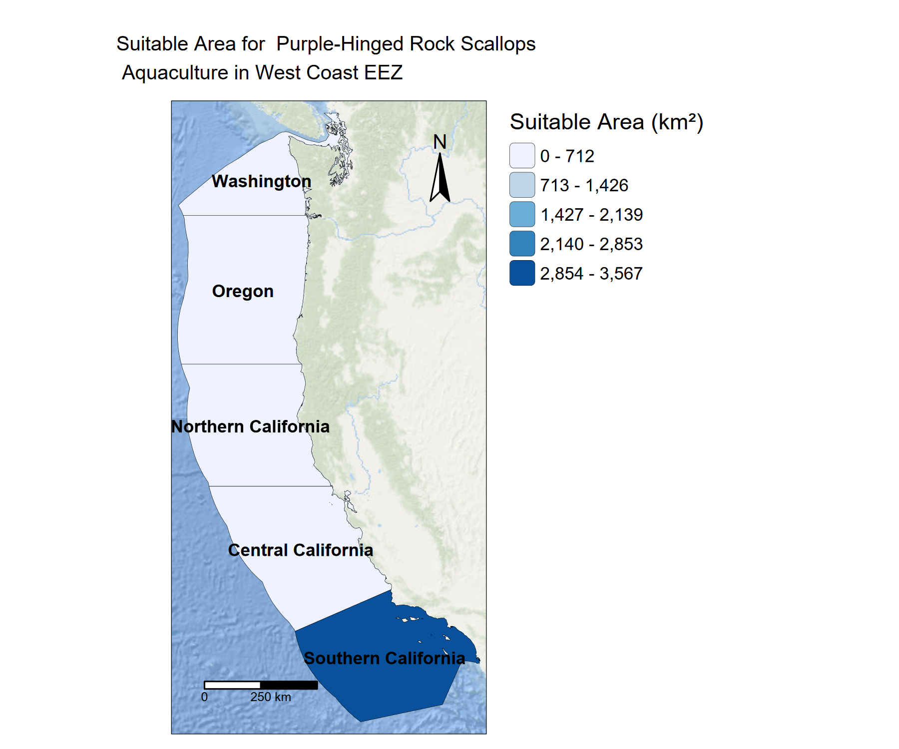
| EEZ Region | Suitable Area (km²) |
|---|---|
| Oregon | 0.0 |
| Northern California | 0.0 |
| Central California | 118.8 |
| Southern California | 3567.3 |
| Washington | 0.0 |
The analysis identified stark differences in the amount of environmentally suitable area for aquaculture across West Coast EEZ regions. For oysters, Central California and Southern California contained the largest suitable areas, with approximately 4,070 squared km and 3,757 squared km respectively, followed by Washington (2,378 squared km) and Oregon (1,074 squared km). Northern California showed a more limited suitable habitat (178 squared km). In contrast, suitable areas for purple-hinged rock scallops were highly concentrated in the southern portion of the study region. Southern California accounted for nearly all suitable habitat (3,567 squared km), with a small area in Central California (119 km²), while Oregon, Washington, and Northern California contained no suitable area based on the species’ temperature and depth thresholds.
The results directly address the project objective of identifying where environmental conditions along the U.S. West Coast support sustainable marine aquaculture development. The spatial differences in aquaculture suitability among oysters and scallops reflect how environmental constraints, namely sea surface temperature and bathymetry, shape the feasibility of expanding aquaculture across Exclusive Economic Zones (EEZs).
Oyster suitability was broadly distributed across the West Coast, with the greatest concentrations being in Central and Southern California. These regions offer both the depth and thermal ranges that align with oyster tolerance, which resulted in several thousand square kilometers of potentially viable habitat. Washington and Oregon also contained meaningful amounts of suitable area, although to a lesser extent. The distribution pattern suggests that oyster aquaculture has relatively flexible environmental requirements within this coastline. This widespread distribution supports prior findings that physical ocean space is unlikely to limit aquaculture expansion (Gentry et al., 2017) and suggests that oysters represent a species with strong potential to contribute to meeting growing seafood demand while alleviating pressure on wild fisheries.
In contrast, the distribution of suitable habitat for purple-hinged rock scallops was highly geographically restricted. Southern California dominated the available area, as it contributed to nearly all suitable habitat identified in the study, with only a small area in Central California meeting threshold conditions. The absence of suitable areas in Oregon, Washington, and Northern California indicates that the species’ temperature range limits its potential along the cooler northern waters. These results align with the species’ known geographic distribution, as purple-hinged rock scallops are more frequently associated with subtidal, subtropical environments (Culver et al., 2022).
The stark contrast between the two species underscores the importance of evaluating on a species-specific level and considering their environmental thresholds when evaluating aquaculture potential. While oysters exhibit broad tolerance across the West Coast that enables aquaculture development across multiple EEZs, the purple-hinged rock scallop is limited to a much smaller geographic range despite being native to the region. From a planning perspective, this means that opportunities to expand scallop aquaculture are highly geographically concentrated, while oyster aquaculture can be distributed more widely. Further research is needed to translate these metrics into practical site selection, like evaluating regulatory conditions, ecological interactions, and infrastructure considerations. Nonetheless, by identifying where environmental conditions are most favorable, this study provides a necessary first step toward supporting sustainable marine aquaculture development along the U.S. West Coast.
Culver, C., Jackson, M., Davis, J., Vadopalas, B., Bills, M., Olin, P., & CENTER, W. R. A. (2022). Advances in purple-hinge rock scallop culture on the US West Coast. Western Regional Aquaculture Center. United States Department of Agriculture, National Institute of Food and Agriculture.
Gentry, R. R., Froehlich, H. E., Grimm D., Kareiva, P., Parke, M., Rust, M., Gaines, S. D., & Halpern, B. S.(2017). Mapping the global potential for marine aquaculture. Nature ecology & evolution, 1(9), 1317-1324.
Harbo, R. M. (1997). Shells & shellfish of the Pacific northwest: a field guide. Madiera Park, BC: Harbour Publishing.
National Oceanic and Atmospheric Administration. (2024). What is an exclusive economic zone (EEZ)? NOAA Ocean Service. Retrieved December 12, 2025, from https://oceanservice.noaa.gov/facts/eez.html
Schmid, J. (2025). Crassadoma gigantea. Retrieved November 30, 2025, from Reef Species of the World website: https://reeflifesurvey.com/species/crassadoma-gigantea/
University of British Columbia. (2025). Crassadoma gigantea, Giant rock-scallop : fisheries. Retrieved November 30, 2025, from Sealifebase.ca website: https://www.sealifebase.ca/summary/SpeciesSummary.php?id=47314&lang=english
NOAA Sea Surface Temperature (SST)
National Oceanic and Atmospheric Administration (NOAA). 2024. 5km Daily Global Satellite Sea Surface Temperature Anomaly v3.1. Coral Reef Watch Program. Average annual SST rasters for 2008–2012 were used in this analysis. Data files: average_annual_sst_2008.tif, average_annual_sst_2009.tif, average_annual_sst_2010.tif, average_annual_sst_2011.tif, average_annual_sst_2012.tif. Available at:
GEBCO Bathymetry
General Bathymetric Chart of the Oceans (GEBCO). 2023. GEBCO Compilation Group: GEBCO 2023 Grid. British Oceanographic Data Centre. Data file: depth.tif. Available at:
Exclusive Economic Zones (EEZ)
Flanders Marine Institute (VLIZ). 2023. Maritime Boundaries Geodatabase: Exclusive Economic Zones (EEZ), version 12. MarineRegions.org. Data file: wc_regions_clean.shp. Available at: